Output files and plotting

Convergence history

When an optimization is carried out with MANGO, an output file is created which records the history of the objective function evaluations. Usually this file is named mango_out.<something>, but any name you like can be set using mango::Problem::set_output_filename. The first 5 lines of this file are header lines, with lines 1, 3, and 5 just a description of what follows. Line 2 is either standard or least_squares, depending on whether the optimization problem has least-squares form. Line 4 gives N_parameters, the dimension of the search space. In the main data section that begins on line 6, the following data are recorded. The objective function evaluation count, the time in seconds since the optimization began, the values of the independent variables, and the value of the objective function. For least-squares problems, additional columns may be included that give the value of each residual term in the objective function. These additional columns can be included or excluded using mango::Least_squares_problem::set_print_residuals_in_output_file.

If the optimization completes gracefully, a final row will be appended to the output file, which is a copy of the previous line corresponding to the minimum objective function.

The data in the output file can be plotted using the python script plotting/mangoPlot. This script requires numpy and matplotlib. As command-line arguments to this script, you can supply the names of one or more MANGO output files. The wildcard character * can be used to select multiple files, just as for commands like ls. The mangoPlot script will display two plots. In both figures, the vertical axis is the objective function minus the minimum value of the objective function found among all the output files being plotted. In the top figure, the horizontal axis is the number of evaluations of the objective function. In the second figure, the horizontal axis is the wallclock time in seconds.

The mangoPlot script is useful for comparing the performance of different optimization algorithms. For example, here is typical output of mangoPlot, comparing 3 PETSc algorithms for the chwirut_c example, each using 5 MPI processors and 5 worker groups:

Levenberg-Marquardt history

When MANGO's native Levenberg-Marquardt algorithm is used, an additional output file is saved containing details of the algorithm's history. The file has the same name as MANGO's main output file described in the previous section, but with _levenberg_marquardt appended. The first row is a header line that labels the columns. Each row thereafter indicates one step in the Levenberg-Marquardt iterations. In this main data, the first column indicates the main (i.e. outer) iteration. The next column, j_line_search indicates the inner iteration, in which the objective function is evaluated in parallel for a batch of values of \(\lambda\). The next N_line_search columns give the values of \(\lambda\) used for these concurrent evaluations. Next come N_line_search columns with the corresponding values of the objective function. The penultimate column gives the 0-based index among these N_line_search values for which the objective function is lowest. The final column is a 0 or 1, indicating whether any of the evaluations in this row successfully reduced the objective function compared to the previous outer iteration.

If the algorithm is working well, the last column should be mostly 1, except at the last outer iteration when the iteration reaches the optimum. Values of 1 mean the range of \(\lambda\) is appropriate, such that the objective function is reduced in the first set of concurrent function evaluations, and further rounds of objective function evaluations are not needed.

The data in one of these Levenberg-Marquardt history files can be plotted with the python script plotting/LevenbergMarquardtPlot. This script requires numpy and matplotlib. The script requires one command-line argument, the name of the _levenberg_marquardt file. Here is an example of typical output, showing a case with N_line_search=8 (corresponding here to the number of worker groups):

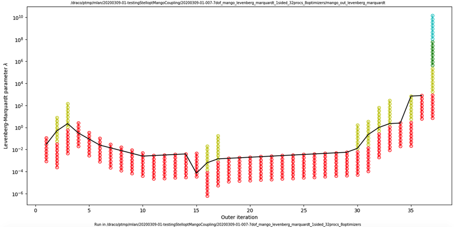
The vertical coordinate is \(\lambda\). Each colored circle represents an evaluation of the objective function, and each column of circles reprents an outer iteration. Colors indicate the inner iteration index j_line_search. In each column, the red batch of points are evaluated concurrently, then the yellow batch of points are evaluated concurrently, etc. The black curve connects the function evaluations with lowest value of the objective function, i.e. the evaluations that were used as the basis for the next outer iteration. Overall, the figure shows how \(\lambda\) evolves during the optimization, and the range of values of \(\lambda\) that are sampled.