Typical usage
Overview
From the Theory and numerical implementation section, we see that the input quantities to the transformation are the following. To compute \(\nu\) (the difference between the old and new toroidal angle) we need \(\iota\), \(\lambda\), \(B_{\theta_0}\), and \(B_{\zeta_0}\). Also we need any scalars that we wish to transform from the old coordinates to the new ones, typically \(R\), \(Z\), and \(B\). All of these quantities must be supplied on each magnetic surface for which we want to execute the transformation.
A common situation is that these input quantities are known on many
magnetic surfaces, but we only wish to execute the transformation on a
subset of the surfaces. For this reason, there are two radial grids
in booz_xform. First, there is a grid for input quantities, with
ns_in surfaces, for which the
normalized toroidal flux has values
s_in. Second, there is a generally
different grid for output quantities, with
ns_b surfaces. The 0-based
indices of the input radial grid on which the transformation will be
executed is determined by
compute_surfs, a vector of
integers. If any radial interpolation of the input data needs to be
done, it should be done before setting the input data on the
ns_in grid; no radial
interpolation is performed during the transformation itself. For
input from a VMEC wout file, radial interpolation from full-grid
quantities to the half-grid is automatically performed by the
read_wout() or
init_from_vmec() functions when
they set the input arrays.
For the input and output quantities that vary on a flux surface, the
dependence on the poloidal and toroidal angles is represented using a
double Fourier series. There are three different Fourier resolutions
used in the code. The input data for \(R\), \(Z\), and
\(\lambda\) use poloidal mode numbers
xm and toroidal mode numbers
xn, with a total of
mnmax modes. The input data for
\(B_{\theta_0}\), \(B_{\zeta_0}\), and \(B\) use poloidal
mode numbers xm_nyq and toroidal
mode numbers xn_nyq, with a total
of mnmax_nyq modes. These two
resolutions could be the same, but they are allowed to be different in
case some quantities are known with different resolution than the others,
as is the case in VMEC. Finally, output quantities (functions of the Boozer angles)
are computed using
poloidal mode numbers
xm_b and toroidal mode numbers
xn_b, with a total of
mnmax_b modes.
This third Fourier resolution is controlled by specifying the maximum poloidal mode number
mpol_b and the maximum toroidal mode number
ntor_b.
Python
Here we show how to drive the Boozer coordinate transformation from python. A similar demonstration can be found in Jupyter notebook form in the repository.
We start by importing the package and creating a Booz_xform object:
>>> import booz_xform as bx
>>> b = bx.Booz_xform()
If desired, we can set the input data directly from python, without a VMEC file:
>>> b.rmnc = [[1, 0.1], [1.1, 0.2]]
Or, we can load in data from a VMEC wout_*.nc file:
>>> b.read_wout("../tests/test_files/wout_li383_1.4m.nc")
We now have access to all the data that was loaded, in the form of numpy arrays:
>>> b.rmnc
array([[ 1.47265784e+00,  1.47064413e+00,  1.46876563e+00, ...,
       1.38298775e+00,  1.38106309e+00,  1.37915239e+00],
     [ 9.66386163e-02,  9.39656679e-02,  9.12856961e-02, ...,
       8.39222860e-04, -1.15483564e-03, -3.14856274e-03],
     [ 5.94466624e-03,  5.33733834e-03,  4.72596296e-03, ...,
      -3.90319604e-03, -3.99352196e-03, -4.08841769e-03],
     ...,
     [ 3.82105109e-07,  1.56748891e-06,  4.30513328e-06, ...,
      -4.47161579e-07, -4.73285221e-07, -2.08934612e-07],
     [-3.72242588e-07, -2.86176654e-06, -6.26756380e-06, ...,
      -7.09993720e-06, -4.03495548e-06, -1.29908981e-06],
     [ 7.68276658e-08, -7.96425120e-08,  7.05128633e-08, ...,
      -9.91504287e-06, -6.37379506e-06, -2.21053463e-06]])
We can set the desired Fourier resolution:
>>> b.mboz = 54
>>> b.nboz = 32
The transformation to Boozer coordinates will be run on all flux surfaces by default:
>>> b.compute_surfs
array([ 0,  1,  2,  3,  4,  5,  6,  7,  8,  9, 10, 11, 12, 13, 14, 15, 16,
     17, 18, 19, 20, 21, 22, 23, 24, 25, 26, 27, 28, 29, 30, 31, 32, 33,
     34, 35, 36, 37, 38, 39, 40, 41, 42, 43, 44, 45, 46, 47],
    dtype=int32)
If desired, we can select only specific surfaces:
>>> b.compute_surfs = [0, 1, 2, 23, 47]
Now, run the calculation:
>>> b.run()
Initializing with mboz=54, nboz=9
nu = 218, nv = 38
             OUTBOARD (theta=0)        SURFACE         INBOARD (theta=pi)
------------------------------------------------------------------------------
zeta    |B|input  |B|Boozer    Error            |B|input  |B|Boozer    Error

  0    1.526e+00  1.526e+00  1.931e-08    0    1.571e+00  1.571e+00  1.100e-08
 pi    1.527e+00  1.527e+00  2.879e-08         1.567e+00  1.567e+00  2.006e-08
  0    1.510e+00  1.510e+00  1.681e-07    1    1.588e+00  1.588e+00  1.468e-09
 pi    1.511e+00  1.511e+00  3.346e-07         1.581e+00  1.581e+00  8.609e-10
  0    1.500e+00  1.500e+00  2.377e-07    2    1.599e+00  1.599e+00  2.861e-09
 pi    1.500e+00  1.500e+00  4.647e-07         1.591e+00  1.591e+00  4.037e-09
  0    1.424e+00  1.424e+00  2.494e-06   23    1.728e+00  1.728e+00  2.405e-07
 pi    1.387e+00  1.387e+00  5.532e-06         1.702e+00  1.702e+00  1.672e-07
  0    1.419e+00  1.419e+00  1.599e-05   47    1.843e+00  1.843e+00  7.609e-06
 pi    1.313e+00  1.313e+00  1.189e-05         1.824e+00  1.824e+00  2.558e-05
(The output can be suppressed by setting b.verbose = False
beforehand.) All of the output data are now available as numpy
arrays:
>>> b.bmnc_b
array([[ 1.54860454e+00,  1.54995067e+00,  1.55126119e+00,
       1.60164563e+00,  1.68603124e+00],
     [ 4.76751287e-04,  2.52763362e-04,  1.02340154e-04,
      -1.06088199e-03,  3.35055745e-03],
     [ 4.55391623e-04,  2.91930336e-04,  1.55133171e-04,
      -1.24795854e-03, -1.46200165e-03],
     ...,
     [-4.75912238e-16,  1.34267428e-16,  1.03266022e-16,
       1.96786082e-16,  2.22042269e-12],
     [-3.33107565e-16, -1.97079156e-16, -4.52095365e-17,
      -2.00845700e-16,  8.16904959e-13],
     [-7.15099095e-17, -1.25428639e-17,  1.70490792e-16,
       1.08711597e-16,  3.86347018e-13]])
The python module includes routines for plotting the results, as described in detail on the Plotting page:
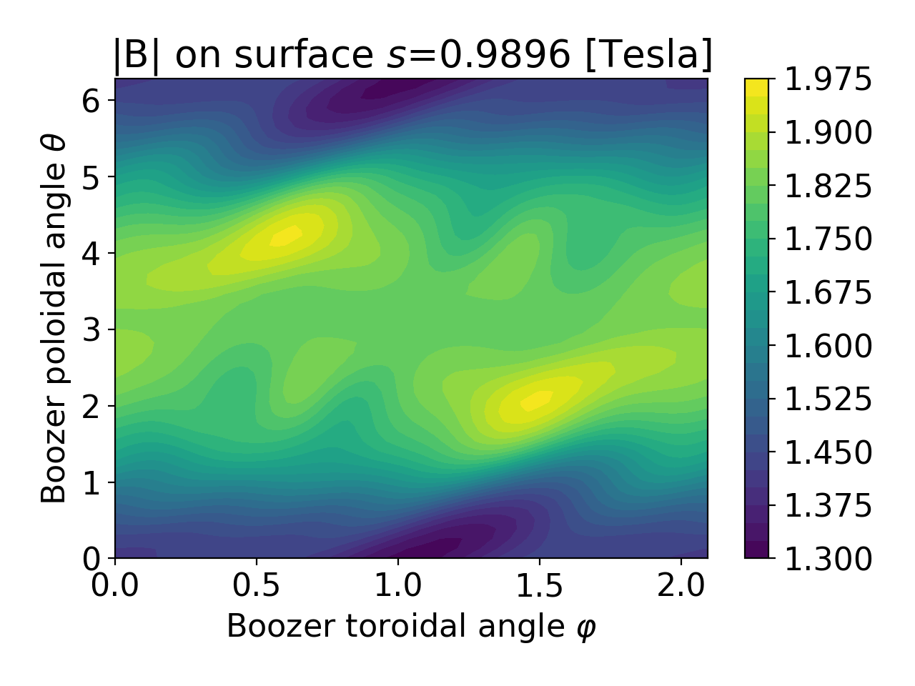
>>> bx.surfplot(b, js=4)
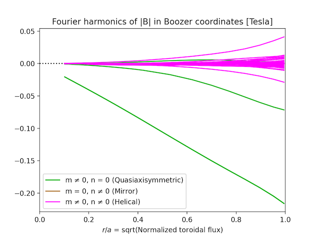
For plots vs. radius, the x axis can be either the normalized toroidal flux \(s\) or \(\sqrt{s}\), and the y axis can be either linear or logarithmic. The \(m=n=0\) mode can be included or excluded.
>>> bx.symplot(b, log=False, sqrts=True, B0=False)
If desired, results can be saved to a boozmn_*.nc NetCDF file:
>>> b.write_boozmn("boozmn_li383_1.4m.nc")
Results from this new booz_xform module are identical to the old
fortran77 version to machine precision:
>>> import numpy as np
>>> from scipy.io import netcdf_file
>>> # Load reference data generated by the F77 version
>>> f = netcdf_file("../tests/test_files/boozmn_li383_1.4m.nc", mmap=False)
>>> bmnc_b_old = f.variables["bmnc_b"][()].transpose()
>>> print("Difference between fortran and C++/python:", np.max(np.abs(bmnc_b_old - b.bmnc_b)))
Difference between fortran and C++/python: 1.021405182655144e-14
C++
For an example of driving the Boozer coordinate transformation directly from C++, without any involvement of python, you can see driver.cpp in the repository.
The first step is to create a Booz_xform object:
booz_xform::Booz_xform b;
All the input data can be read in from a VMEC wout file:
b.read_wout("wout_li383_1.4m.nc");
However it is not necessary to use a VMEC file. Instead, the input data can be set directly. 1D and 2D arrays use the Eigen package, as discussed in more detail in the API Reference.
b.mnmax = 100;
b.ns_in = 51;
b.rmnc.resize(b.mnmax, b.ns_in);
b.rmnc(3, 5) = 0.013;
You may wish to set the resolution, and choose which surfaces on which to run the transformation.
b.mboz = 54;
b.nboz = 32;
b.compute_surfs.resize(1);
b.compute_surfs[0] = 47;
The transformation is run using
b.run();
You may wish to save the results to a NetCDF file, though this is not mandatory:
b.write_boozmn("boozmn_li383_1.4m.nc");
All of the output data are also available directly from the member variables of the class instance:
std::cout << "B(0,0): " << b.bmnc_b(0, 0) << std::endl;